Regarding the importance of exponential quantum advantages, it is natural to ask how far the boundaries of known, superfast quantum algorithms may be pushed. In the case of quantum computing‘s most famous algorithm, Shor’s algorithm, this leads to the quantum computing frameworks for the “Hidden Subgroup Problem” and generalized Fourier transform. Instances of this range from hidden shift, integer period finding, discrete logarithm up to lattice cryptosystems and graph isomorphism. Unfortunately, the search for introductions quickly leads to very demanding “LaTeX deserts” and paper cascades.
This article provides a gentle and intuitive introduction and a broad overview to the very fascinating and elegant subject.
Image by Matthias Wewering from Pixabay
Contents
- 1 The importance of Exponential Quantum Advantages
- 2 Simon’s Problem, a Hidden Subgroup Problem
- 3 The general Hidden Subgroup Problem
- 4 The Hidden Subgroup Problem for Abelian groups
- 4.1 Some rules for irreducible representations and characters
- 4.2 Quantum Fourier Transform: The centerpiece of the Hidden Subgroup Problem
- 4.3 Shift-Operators for $G$
- 4.4 The Fourier transform for $ G $
- 4.5 Fourier transform for $ \mathbb{Z}_m $ , $ \mathbb{Z}_2^n $ and the magical 2nd Hadamard
- 4.6 The Forrelation Problem
- 4.7 Tackling the coset state
- 4.8 Constraints for the Fourier labels
- 4.9 Fourier sampling the coset state
- 4.10 Example: Shor’s Algorithm as a Hidden Subgroup Problem
- 5 The Hidden Subgroup Problem for non-Abelian groups
- 5.1 Graph Isomorphism as a Hidden Subgroup Problem
- 5.2 A Fourier-like basis for non-Abelian groups
- 5.3 Strong Fourier Sampling
- 5.4 Weak Fourier Sampling
- 5.5 Limits of Fourier Sampling
- 5.6 The Hidden Subgroup Problem for Dihedral Groups
- 5.7 Example: Fourier Sampling the Dihedral Group D4
- 5.8 Entangled measurements and the Kuperberg sieve
- 5.9 Lattice cryptography and the Dihedral Hidden Subgroup Problem
- 6 Appendix 1: Some facts about group and representation theory
- 7 Appendix 2: Fourier sampling the abelian coset state in detail
- 8 Appendix 3: Strong and Weak Fourier sampling in detail
- 9 Footnotes
1 The importance of Exponential Quantum Advantages
As quantum computing evolves the community starts to focus on the next steps towards fault tolerance. These developments start to highlight an aspect that is often overlooked: The algorithmic overhead of fault tolerance. In my last article Does Quadratic Quantum Speedup have a problem? I described two papers that formulate concerns regarding central quantum algorithms with small polynomial speedup in comparison to its classical counterparts.
Also because of this outlook, leading scientists in quantum computing like Scott Aaronson, emphasize the importance of exponential asymptotics to quickly reach the breakeven time with classical algorithms. In his talk at the Solvay Physics Conference (May 2022, Brussels) he gives a very informative overview about the current state of exponential quantum advantage i. Here I want to spoil just one thing from the very readable transcript: After summarizing some of the known exponential speedups, he concludes “People often ask, is that it? Well, it’s not quite it, but yes: the list of exponential speedups is smaller and more specialized than many people would like”.
In this light, it is reasonable to ask the question: How far may the boundaries of the known, superfast quantum algorithms be pushed?
Now quick! What’s the very first quantum computing algorithm that comes to your mind now?
1.1 From Shor to the Hidden Subgroup Problem
Let me guess, it’s Shor’s algorithm, the mother of all quantum computing algorithm? … OK, presumably. But let’s face it: Shor’s algorithm for factoring prime numbers not only sparked all the great attention for quantum computing – and does so until today! More importantly, it brilliantly condenses crucial aspects and subroutines of quantum computing into one single algorithm. Having done this already in the year 1994 was Peter Shor’s farsighted masterpiece for science and he was justifiably honored with the Breakthrough Prize 2023 for it. Besides, until now it serves as a centerpiece for various (rather constructed) use cases with an exponential quantum advantages. Namely for use cases in optimization ii or in machine learning iii, for which you usually find rather quadratic speedups.
Taking Shor’s algorithm even further we end up with the quantum computing framework for the Hidden Subgroup Problem.
Among its instances are
- Finding hidden shifts in bitstring functions (also known as “Simon’s Problem”)
- Period finding over integers (the core of Shor’s factoring algorithm)
- Discrete logarithm
- Lattice cryptosystems (Regev’s algorithm)
- Graph isomorphism
The hidden subgroup problem is very often referred to as one of the major applications for quantum computing. But if you want to get ready for a deeper dive into the subject you are quickly lost in cascades of papers and very demanding LaTeX deserts: “Ehh … ok … let’s save this up for later.”
Which is really a shame, because the hidden subgroup problem is a highly fascinating subject. Also, its quantum computing framework is mathematically very elegant and what seems rather technical in Shor’s or Simon’s algorithm, has a deeper and intuitive reason. My article aims to provide a gentle and intuitive introduction and a comprehensive overview to the very fascinating but challenging subject. Of course, I will also use some math – quite a bit actually – but I will emphasize the crucial points and the intuition in the main text and provide much more helpful comments than you would usually find. Purely technical details are rather presented in the appendices. Besides this, I will outline the most interesting examples of the hidden subgroup problem and point out some limits of the framework.
Ok, let’s start our tour.
It all began with Simon’s problem …
2 Simon’s Problem, a Hidden Subgroup Problem
As stated by Peter Shor, he was heavily inspired by Simon’s algorithm which is the simplest solution of a hidden subgroup problem. Daniel Simon’s introduced the problem in 1994 and proved for the first time, that there exists an exponential oracle separation between classical and quantum computing: A quantum algorithm is able to query a black box function exponentially fewer times than the classical counterpart to solve the problem. Recently Simon’s problem was even adapted to the NISQ regime, proving for the first time, that the exponential oracle-speedup holds even for noisy near term quantum computers iv. Here I will quickly recap Simon’s algorithm and point out some crucial basic aspects that you will later recognize again, in a much more abstract form in the quantum computing framework for the hidden subgroup problem. I will heavily make use of the very nice introduction to Simon’s algorithm in IBM’s great Qiskit textbook v.
2.1 Simon’s Algorithm to solve the Hidden Shift Problem
Image by Gerd Altmann from Pixabay
We are given an unknown blackbox function $f$ for bitstrings of size $n$, which is two-to-one and the additional promise of a unique hidden bitstring $b$:
\begin{gather}
\textrm{given }x_1,x_2: \quad f(x_1) = f(x_2) \\
\textrm{it is guaranteed }: \quad x_1 \oplus b = x_2
\end{gather}
where $ x_1 \oplus b $ is of course the modulo binary addition for bitstrings.
Problem: Find the hidden bitstring $ b $!
The classical solution is exponentially hard, because in the worst case you might need to execute the blackbox function for half of the exponentially many bitstrings $ x_i $ until you complete a pair. On average you have to execute half as many bitstrings which are still exponentially many.
In the quantum computing version you need to execute the blackbox function only $n$ times!
We achieve this, using an iterated approach with the following steps in each iteration:
- We initialize two $n$-qubit input registers to the zero state:\begin{gather}\lvert \psi_1 \rangle = \lvert 0 \rangle^{\otimes n} \lvert 0 \rangle^{\otimes n}\end{gather}
- We apply a (first) Hadamard transform to the first register, which generates a uniform superposition of all possible bitstrings:\begin{gather}\lvert \psi_2 \rangle = \frac{1}{\sqrt{2^n}} \sum_{x \in \{0,1\}^{n} } \lvert x \rangle\lvert 0 \rangle^{\otimes n}\end{gather}
- We apply a controlled operation which executes the query function via composed gates $\text{Q}_f$ on the second register:\begin{gather}\lvert \psi_3 \rangle = \frac{1}{\sqrt{2^n}} \sum_{x \in \{0,1\}^{n} } \lvert x \rangle \lvert f(x) \rangle\end{gather}
- We measure the second register. A certain value of $f(x)$ will be observed. Because of the setting of the problem, the observed value $f(x)$ could correspond only to two possible inputs: $x_1$ and $x_2 = x_1 \oplus b $. Therefore the first register becomes:
\begin{gather}\lvert \psi_4 \rangle = \frac{1}{\sqrt{2}} \left( \lvert x_1 \rangle + \lvert x_1 \oplus b \rangle \right)
\end{gather}
We omitted the second register since it has been measured and we don’t care for its value. All we needed was, that the first register collapsed into a superposition of a single pair linked by the hidden bitstring $b$. Now, we would like to find some way to get rid off $x_1$. - We magically guess that a second Hadamard on the first register might help. For this it is helpful to remember the “definition” of a general Hadamard transform for a bitstring $x$:\begin{gather}H \lvert x \rangle = \frac{1}{\sqrt{2^{n}}} \sum_{z \in \{0,1\}^{n} } (-1)^{x \cdot z} \lvert z \rangle\end{gather}where $ x \cdot z $ is the inner product of the two bitstrings / binary vectors. In this case, we get
\begin{gather}\lvert \psi_5 \rangle = \frac{1}{\sqrt{2^{n}}} \sum_{z \in \{0,1\}^{n} } \left[ (-1)^{x _1 \cdot z} + (-1)^{(x_1 \oplus b) \cdot z} \right] \lvert z \rangle
\end{gather}We will later find out exactly why a second Hadarmard transform was just the right thing for this purpose. You will be surprised! - Now we measure the first register. It will give us an output only if:\begin{gather}(-1)^{x_1 \cdot z} = (-1)^{(x_1 \oplus b) \cdot z}\end{gather}which means:\begin{gather}x_1 \cdot z = \left( x_1 \oplus b \right) \cdot z \\
x_1 \cdot z = x_1 \cdot z \oplus b \cdot z \\
b \cdot z = 0 \text{ (mod 2)}
\end{gather}Like I promised: We got rid off the $ x_1 $!We see, that we will measure a bitstring $z$, whose inner product with $b$ gives $0$. Thus, repeating the algorithm $\approx n$ times, we will be able to obtain $n$ different bitstrings $z_k$ and the following system of equation can be written:\begin{gather}
\begin{cases} b \cdot z_1 = 0 \\ b \cdot z_2 = 0 \\ \quad \vdots \\ b \cdot z_n = 0 \end{cases}
\end{gather}From which $b$ can be determined, for example by Gaussian elimination.
2.2 What is the deal with the black box function?
The use of black box functions / oracles seems mysterious at first as these are just algorithmic sub routines. The whole point is, that usually one cannot rule out an efficient classical solution, if details are known about the concrete problem structure. If we limit ourselves to being ignorant, there is no way to exploit any structure and to take shortcuts. If we are forced to execute the black box function many, many times, it enables us to separate the complexity of quantum and classical solutions – relative to the oracle – and thus differentiate between the nature of quantum computing and classical computation.
Yet, in certain cases it is possible to extend the relative advantage to an absolute advantage. like in Shor’s algorithm. A necessary condition for this is, that the oracle needs to be efficiently computable. This is not always possible, just for the simple reason, that there are vastly more possible oracles than there are efficient computations. Finding such absolute examples for Simon’s problem would make them great candidates for near term quantum supremacy experiments. Unfortunately this is an open question.
2.3 The Connection to the Hidden Subgroup Problem
Here are some crucial remarks to Simon’s algorithm in the context of the hidden subgroup problem:
The steps 1-4 seem kind of straight forward. The magic is happening in steps 5 and 6. After the measurement of the second register we created the uniform superposition
\begin{gather}
\frac{1}{\sqrt{2}} \left( \lvert x_1 \rangle + \lvert x_1 \oplus b \rangle \right)
= \frac{1}{\sqrt{2}} \left( \lvert x_1 \oplus 0 \rangle + \lvert x_1 \oplus b \rangle \right)
\end{gather}
We may symbolically write this as
\begin{gather} \lvert x_1 \oplus H \rangle
\quad \textrm{for the set } \quad
H = \bigl\{0, b \bigr\}
\end{gather}
Notice, that
\begin{gather}
b \oplus b = 0 \quad \textrm{making H … a group!}
\end{gather}
Of course, we will exploit this fact further down. By the way: As you might have guessed already $H$ is even a subgroup of a certain other group.
Next, we still have to find out what is the deal with the second Hadamard transform. I leave this for later, too.
Now, just for fun, let’s call
\begin{gather}
\bigl(-1\bigr)^{x \cdot z} = \chi_z(x) \quad \textrm{a “character function”.}
\end{gather}
We notice, that after step 6, the final measurement collapses the previous superposition to only those “labels” $ z $ for which the character $ \chi_z $ is constant on the complete set $ x_1 + H $! As we will see, these $ \chi_z $ are even equal to the trivial character on the domain $ H $
\begin{gather}
\chi_z(x) = \bigl(-1\bigr)^{x \cdot z} = 1
\end{gather}
We got rid off $ x_1 $ because every character function $ \chi_z $ has the nice property
\begin{gather}
\chi_z (x_1 + x_2) = \chi_z (x_1) \cdot \chi_z (x_2) \quad \textrm{for all } x
\end{gather}
This property makes $ \chi_z $ a “group homomorphism”.
At the end we are able to extract the group $ H $ because:
- We somehow guessed the exact form of the characters. These seemed to be kind of native to this type of problem.
- We knew, that the final measurement only gave us those labels, for which the corresponding character is trivial on the set $ H $
- Repeating this iteration gives us more and more information about $ H $ and we are able to efficiently compute it classically.
3 The general Hidden Subgroup Problem
Now we are ready to formulate the Hidden Subgroup Problem itself:
We are given a group $ G $ and a function $f$ from $ G $ to some set $ X $:
\begin{gather}
f: G \longrightarrow X
\end{gather}
Further we are told, that $ f $ has the unique feature, that there is a hidden subgroup $ H \subseteq G $ on which $ f $ is “H-periodic”:
\begin{gather}
\textrm{for every $ g_1, g_2 $ with:} \quad f(g_1) = f(g_2) \\
\textrm{it is guaranteed that:}
\quad g_1 \cdot h = g_2 \\
\textrm{for a $ h \in H $}
\end{gather}
In other words: $ f $ is constant exactly on every “coset” $ S_i := g_i \cdot H $ with distinct values for every distinct coset $ S_i $.
Problem: Find the hidden subgroup $ H $!
In the following sections we will
- See how to create so called “coset states” for the general problem
- First solve the problem for abelian / commuting groups
- Consider the hidden subgroup problem for non-abelian groups
- Discuss some examples
3.1 The Quantum Algorithm for the Hidden Subgroup Problem
First of all, to do quantum computation, we need to encode the problem into a Hilbert space.
For this, we map the group $ G $ to a Hilbert space of dimension $ |G| $ (the number of elements in $G$) by identifying each group element with a basis vector of the standard basis:
\begin{gather}
\{ \lvert g \rangle: g \in G \}
\end{gather}
(By the way: This also defines the “regular representation” of $G$)
All the group operations in $G$ are now encoded in a set of shifting operators (left shift and right shift to b e exact):
\begin{gather}
U_l(k): \lvert g \rangle \longrightarrow \lvert k \cdot g \rangle \quad g, k \in G
\end{gather}
We will exploit this fact further down.
To solve the hidden subgroup problem, we start just like in Simon’s problem.
- We initialize two input registers to the zero state:\begin{gather}\lvert \psi_1 \rangle = \lvert 0 \rangle^{\otimes n} \lvert 0 \rangle^{\otimes m}\end{gather}The actual dimensions $n$ and $m$ of the two registers are adapted to $|G|$ and the image of $ f(G) $
- We apply a Hadamard transform to the first register, which creates a uniform superposition over all group elements,\begin{gather}\lvert \psi_2 \rangle = \frac{1}{\sqrt{|G|}} \sum_{g \in G } \lvert g \rangle\lvert 0 \rangle^{\otimes m}\end{gather}
- We apply a controlled operation which executes the query function via composed gates $\text{Q}_f$ on the second register:\begin{gather}\lvert \psi_3 \rangle = \frac{1}{\sqrt{|G|}} \sum_{g \in G} \lvert g \rangle \lvert f(g) \rangle\end{gather}
- We measure the second register. A certain value of $f(g)$ will be observed. Because of the setting of the problem, the observed value $f(g)$ could correspond only to inputs in the (left) coset $ S = g \cdot H $. Therefore the first register becomes:\begin{gather}\lvert \psi_4 \rangle = \frac{1}{\sqrt{|H|}} \sum_{h \in H} \lvert g \cdot h \rangle =: \lvert g \cdot H \rangle
\end{gather}
We omitted the second register since it has been measured and we don’t care for its value. All we needed, was that the first register collapsed into the so called “coset state”.
Now we are stuck! We don’t know how to extract $ H $ from the coset state. This is really too bad. Measuring this state won’t do, because we don’t know $ g $ and each iteration would randomly give us another one.
To solve this problem we need a few tools and rules from abstract algebra.
I promise: This will give you some neat intuition on how to tackle the coset state!
4 The Hidden Subgroup Problem for Abelian groups
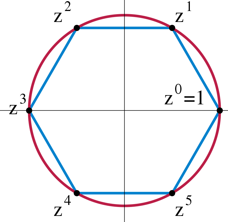
Image by Jakob.scholbach, via Wikimedia
4.1 Some rules for irreducible representations and characters
Tightly connected to the hidden subgroup problem, and may be mathematically even more fascinating, is the question for the Fourier transform on arbitrary groups. For functions (or “vectors”) on the real line (the group of real numbers under ordinary addition) we might already know the regular Fourier transformation. The Fourier transform on arbitrary groups requires a few tools and rules from abstract algebra. If your knowledge about groups and representations feels a little waggy you might want to check out my quick summary “Appendix 1: Some facts about group and representation theory” further down.
But if the following terms only put a smile of wisdom on your face, you will do just fine
- Abelian groups
- Group of bitstrings $ \mathbb{Z}_2^n $
- Cyclic group $ \mathbb{Z_{m}} $
- Cosets
- Representations, Irreducible representations
- Characters
For this and the next section I will stick to the paper of Ekert & Jozsa 1998, “Quantum Algorithms: Entanglement Enhanced Information Processing” vi. Also, we will first deal with the hidden subgroup problem for finite abelian groups and later discuss adaptions to other cases.
Now to some crucial rules for characters: Let $(G, +)$ be any finite abelian group and let’s write the group operation in additive notation. Let $|G|$ be the number of elements of $G$. For abelian groups irreducible representations are 1-dimensional and equal to their traces, their “characters”: So both are functions $\chi$ from $G$ to the complex numbers
\begin{gather}
\chi : G \longrightarrow \mathbb{C}
\end{gather}
with
\begin{gather}
\chi(g_1 + g_2) = \chi(g_1 ) \cdot \chi(g_2)
\end{gather}
i.e. $\chi$ is a group homomorphism. This has the following consequences
- 1. Any value $\chi(g)$ is a $|G|$ th root of unity. Thus $\chi$ may be viewed as a group homomorphism to the complex circle group of all units
\begin{gather}
\chi : G \longrightarrow S^1 = \left\{ e^{i\phi} \right\}
\end{gather}
And in particular: $ \chi \left( g^{-1} \right) = \overline{\chi(g)} $
- 2. Orthogonality (Schur’s lemma): If $\chi_i$ and $\chi_j$ are any two such functions then:
\begin{gather}
\frac{1}{|G|} \sum_{g \in G} \chi_i(g) \cdot \overline{\chi_j(g)} = \delta_{ij}
\end{gather}
- 3. There are always exactly $|G|$ different functions $\chi$ satisfying this. So we may label them by the elements of $ k \in G$: $\chi_k$.
4.2 Quantum Fourier Transform: The centerpiece of the Hidden Subgroup Problem
4.3 Shift-Operators for $G$
Again, we use a Hilbert space of dimension $ |G| $ with the basis:
\begin{gather}
\{ \lvert g \rangle: g \in G \}
\end{gather}
Remember that all group operations in $G$ are now encoded in a set of shifting operators:
\begin{gather}
U(g’): \lvert g \rangle \longrightarrow \lvert g+g’ \rangle \quad g, g’ \in G
\end{gather}
Using all the characters $\chi_k$ of $ G $ with labels $ k \in G $, we introduce a family of very interesting states:
\begin{gather}
\lvert \chi_k \rangle =
\frac{1}{\sqrt{|G|}} \sum_{g \in G} \overline{\chi_k(g)} \cdot \lvert g \rangle
\end{gather}
These states are orthonormal since all characters are orthonormal (see Schur’s lemma in the section above). Furthermore: These states are eigenstates of all translation operators!
\begin{align}
U(g’) \lvert \chi_k \rangle &=
\frac{1}{\sqrt{|G|}} \sum_{g \in G} \overline{\chi_k(g)} \cdot U(g’) \lvert g \rangle \\
&=
\frac{1}{\sqrt{|G|}} \sum_{g \in G} \overline{\chi_k(g)} \cdot \lvert g + g’ \rangle
\end{align}
Since
\begin{gather}
\overline{\chi_k(g)} = \overline{\chi_k(-g’ + g + g’)} = \chi_k(g’) \cdot \overline{\chi_k(g + g’)}
\end{gather}
and we may relabel the sum over all group elements to $ g+g’$ as well. This gives
\begin{gather}
U(g’) \lvert \chi_k \rangle = \frac{1}{\sqrt{|G|}} \cdot \chi_k(g’) \cdot \lvert \chi_k \rangle
\end{gather}
4.4 The Fourier transform for $ G $
May be you have guessed this already:
\begin{gather}
\bigl( \lvert \chi_k \rangle \bigr)_{k \in G} \quad \text{is called the Fourier basis for $ G $.}
\end{gather}
As mentioned, the Fourier states are orthonormal and there are $ |G| $ of them.
The Fourier transform is defined as the map, that extracts the label for each Fourier state:
\begin{gather}
\mathcal{F} \lvert \chi_k \rangle = \lvert k \rangle
\end{gather}
Thus, it translates every state into its spectrum of Fourier labels. In particular we have
\begin{align}
\mathcal{F} &= \sum_{k \in G} \lvert k \rangle \langle \chi_k \lvert \\
&= \frac{1}{\sqrt{|G|}} \cdot \sum_{k, g \in G} \chi_k(g) \lvert k \rangle \langle g \lvert
\end{align}
4.5 Fourier transform for $ \mathbb{Z}_m $ , $ \mathbb{Z}_2^n $ and the magical 2nd Hadamard
As we know that $ \chi_k $ are $ |G| $th roots of the unity, we can start constructing the Fourier transform for different abelian groups.
For the cyclic group $ \mathbb{Z}_m $, there are the following $ m $ roots of unity:
\begin{gather}
\chi_k (g) = e^{ 2\pi i \cdot \frac{k}{m} \cdot g}
\end{gather}
In particular for $ \mathbb{Z}_2 $ we have for the two bits $g$ and $k$
\begin{gather}
\chi_k (g) = e^{ \pi i \cdot k \cdot g} = (-1)^{k \cdot g}
\end{gather}
For $ \mathbb{Z}_2^n $ the $ n $ characters from above just factor and we can sum up the individual exponents. Altogether the two bits turn into two bitstrings and the product $k \cdot g$ in the exponent turns into the inner product of the two bitstrings:
\begin{gather}
\mathcal{F} = \frac{1}{\sqrt{2^{n}}} \sum_{k, g \in \{0,1\}^{n} } (-1)^{k \cdot g} \lvert k \rangle \langle g \lvert
\end{gather}
We have just found our magical second Hadamard transform in the Simon’s algorithm!
4.6 The Forrelation Problem
Just as a side remark: The fact, that the Fourier transform of $ \mathbb{Z}_2^n $ – functions may be implemented on a quantum computer so efficiently, inspired Scott Aaronson, to formulate another black box problem in 2009, the “Forrelation” problem: Given two black box functions $f$, $g$. Is the $ \mathbb{Z}_2^n $-Fourier transform of $ f $ correlated to $ g $ (using a special Fourier-like metric)?
He introduced the problem while trying find an even more spectacular black box separation, the separation between $ BQP $ and the “Polynomial Hierarchy (PH)”. Ten years later R. Raz and A. Tal proved just this, which was a major breakthrough in quantum complexity theory.
There is nice article on Quantamagazine to this (along with further references) vii.
By the way, the Polynomial ierarchy is like exponentiating the class NP further and further. Basically it is similar to $ N \times N $ check. In this sense, NP is like Checkmate in one move. As we climb up the Polynomial hierarchie, the problem gets drastically harder: Checkmate in two moves, Checkmate in three moves, in four moves, … And this would remain hard, even if NP problems were efficiently solvable.
4.7 Tackling the coset state
Now we have set up everything to extract $ H $ from the coset and solve the hidden subgroup problem for finite abelian groups. Let’s recap:
We are given a finite abelian group $ (G, +) $ and a H-periodic black box function $f$ on $ G $ to some set $ X $.
We created a coset state by generating the state
\begin{gather}
\lvert \psi_3 \rangle = \frac{1}{\sqrt{|G|}} \sum_{g \in G} \lvert g \rangle \lvert f(g) \rangle
\end{gather}
and measuring the second register, getting some value $f(g)$. In the first register this leaves:
\begin{gather}
\lvert \psi_4 \rangle = \frac{1}{\sqrt{|H|}} \sum_{h \in H} \lvert g + h \rangle =: \lvert g + H \rangle
\end{gather}
This is the point where we got stuck before, since
\begin{gather}
\lvert g + H \rangle = U(g) \cdot \lvert H \rangle
\end{gather}
and we are only interested in the latter state. But by now we know a G-invariant basis: The Fourier basis. And we know, that $ \lvert H \rangle $ may be written as some superposition in this basis:
\begin{gather}
\lvert H \rangle = \sum_{k \in G} \alpha_k \cdot \lvert \chi_k \rangle
\end{gather}
As all $ \lvert \chi_k \rangle $ are translationally invariant, $ U(g) $ will only add a phase factor to the amplitutes $ \alpha_k $ in this superposition
\begin{gather}
U(g) \cdot \lvert H \rangle = \sum_{k \in G} \chi_k(g) \cdot \alpha_k \cdot \lvert \chi_k \rangle
\end{gather}
You might think: So what? Unfortunately the phase factors are local! But the crucial thing is that $ \lvert g + H \rangle $ and $ \lvert H \rangle $ have the same spectrum of Fourier labels. If we “Fourier sample” the superposition above, it will collapse to a single label $k$, one that is also a label of $ \lvert H \rangle $. Plus, the local phase factor $\chi_k(g)$ does not matter any more, so even the measured probabilities are the same.
This means, we just need to apply a Fourier transform of $G$ on the coset state in the first register and measure the first register.
So we are done, right? Not so fast. There is another surprise waiting!
4.8 Constraints for the Fourier labels
We may actually formulate some crucial constraints for the measured Fourier labels as well:
The same argument from above also applies to every shift by an element $ h \in H $:
\begin{gather}
U(h) \cdot \lvert H \rangle = \sum_{k \in G} \chi_k(h) \cdot \alpha_k \cdot \lvert \chi_k \rangle
\end{gather}
But since $ H $ is a group, we have $ U(h) \cdot \lvert H \rangle = \lvert H \rangle $. For each individual amplitude, this means:
\begin{gather}
\chi_k(h) \cdot \alpha_k = \alpha_k
\end{gather}
This is only possible if
\begin{gather}
\chi_k(h) = 1 \\
\text{or} \\
\alpha_k = 0
\end{gather}
Thus, we will only measure labels of trivial characters on $H$.
4.9 Fourier sampling the coset state
By repeating these steps over and over again we collect more and more of those labels. Since we know $ G $, we know its characters $ \chi_k $. Thus, we gain more and more information about the domain on which all the characters are trivial.
As for every homomorphism, it is guaranteed that each of those “kernels” $\{g \in G: \chi_k(g) = 1\} $ is a subgroup (think about this claim for a second). The intersection $ K $ of all kernels will also be a subgroup (think about this for another second). After only polynomially many steps, the subgroup obtained this way is the hidden subgroup $ H $ with high probability. We will see the reason for this below.
If you want to see the calculation for Fourier sampling the coset state in detail, please check out the “Appendix 2: Fourier sampling the abelian coset state in detail”. There, you will also see that the remaining amplitudes from above are even constant:
\begin{gather}
\alpha_k = \frac{1}{\sqrt{|G| \cdot |H|}} \cdot \sum_{h \in H} \chi_k(h) = \sqrt{\frac{|H|}{|G|}}
\end{gather}
May be this is something, that one could have expected all along, since the Fourier transform is most sensitive to periodic patterns.
In the appendix I followed the presentation in Andrew Childs’ great “Lecture Notes on Quantum Algorithms” (chapter 6) viii.
Childs’ lecture is actually my most favorite course on the quantum computing algorithm landscape. If you haven’t done so far, you should definitely take a closer look at it. It is incredibly comprehensive, up to date and a great starting point to tackle the papers themselves. Yet Childs is also a demanding teacher and you should bring some time with you. But it’s worth it.
He also gives a tricky argument for the efficiency of Fourier sampling coset states for abelian subgroups. The claim is, that each sampling will cut the intersection $ K $ of all kernels $\{g \in G: \chi_k(g) = 1\} $ at least to half with a probability greater than 50%. Thus, $ K $ will shrink exponentially fast to $ H $. I simplified it a little bit with some additional remarks:
As stated above the intersection $ K $ is a subgroup of $ G $ itself. So, either already is $ H = K $ or not yet $ H < K $. If $ H $ is still a proper subgroup of $ K $, Langrange’s theorem tells us more about their sizes:
\begin{gather}
|K| = [K:H] \cdot |H|
\end{gather}
where $ [K:H] $ is the number of distinct cosets, which is at least $ [K:H] \ge 2$. This applies to subgroups in general: A proper subgroup contains at most half of all group elements:
\begin{gather}
|H| \le \frac{1}{2} \cdot |K|
\end{gather}
The same is true for each consecutive intersection $ K $: Each Fourier sampling will either reveal new information and $ K $ will at least cut to half or we don’t gain new information and $ K $ will stay the same. Now, the important question is: What’s the probability for this?
We know from above, that the probability for measuring a certain label is:
\begin{gather}
P(k) = |\alpha_k|^2 = \frac{|H|}{|G|}
\end{gather}
This also means, there are $ \frac{|G|}{|H|} $ labels altogether. How many of those labels will reveal new information and shrink the current intersection $ K $ further? We may answer this by thinking about a different question: What would be the situation if the current intersection $ K $ was the hidden subgroup itself? Then, the number of labels defining $ K $ would be $ \frac{|G|}{|K|} $. Returning to the situation for $ H $, this means, that the probability to Fourier sample a blank (a $ k $ that is among the set of labels defining the intersection $ K $) is
\begin{gather}
P_{\text{blank}} = \frac{|H|}{|G|} \cdot \frac{|G|}{|K|} = \frac{|H|}{|K|} \le \frac{|H|}{2|H|} = \frac{1}{2}
\end{gather}
The opposite to this proves the claim above: The probability to sample a $ k $ which reveals new information is $ > \frac{1}{2} $ !
And by the way, the argumentation also shows: The greater $ K $ is compared to $ H $, the faster will it shrink (even faster than $ \frac{1}{2} $).
4.10 Example: Shor’s Algorithm as a Hidden Subgroup Problem
As this article also deals with Shor’s algorithm, let’s look briefly into it as an example of a hidden subgroup problem (you may find all the details in any introduction of Shor’s algorithm):
$N_0$ is an integer, that we want to prime-factor and this can famously be done by finding the integer period $ r $ for the modular exponentiation of some integer $a < N_0$.
\begin{gather}
f(x) = a^x \text{ mod } N_0 \quad \text{with} \quad f(x) = f(x+r)
\end{gather}
Thus, Shor’s algorithm is an integer period finding algorithm. Looking at it as a hidden subgroup problem, we choose $ G = \mathbb{Z}_N $ with $N$ being some multiple of $r$. It shows, that $N=O(N_0^2)$ is a good choice and we don’t even need a precise multiple of $r$, if $N$ is large enough. We are looking for the hidden subgroup:
\begin{gather}
H = \{0, r, 2r, 3r, …\}
\end{gather}
By now, we are able to immediately write done the character labels $k$, that we will Fourier sample for this type of problem!
Above, we saw that the characters for $ \mathbb{Z}_N $ are:
\begin{gather}
\chi_k(g) = e^{ 2\pi i \cdot k \cdot \frac{g}{N}}
\end{gather}
Sampling only trivial characters on $H$, will give us:
\begin{gather}
\chi_k(r) = \chi_k(2r) = \chi_k(3r) = … = 1 \\
\iff \\
k \text{ is a multiple of } \frac{N}{r}
\end{gather}
Thus, we only need to measure a few $k_1$, $k_2$, … and find their greatest common denominator
\begin{gather}
r = \text{gcd}(k_1, k_2, …)
\end{gather}
That’s it!
5 The Hidden Subgroup Problem for non-Abelian groups
Now, we would like to solve the hidden subgroup problem for finite non-abelian groups $ (G, \cdot) $ as well. It turns out, that this is much more challenging. A very interesting application are lattice cryptosystems which are connected to dihedral groups. I will give some details about this example at the end of this article. Another very interesting application is the problem to decide, if two graphs are isomorphic. As a teaser I will sketch this problem first in the context of the hidden subgroup problem. Afterwards we will get into the details about the quantum computing framework of the hidden subgroup problem for non-abelian groups.
5.1 Graph Isomorphism as a Hidden Subgroup Problem
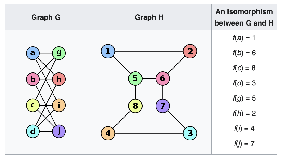
Image by Booyabazooka via Wikimedia
Ok, let’s look at graph isomorphism as a hidden subgroup problem. For this I will follow Richard Jozsa’s description in “Quantum factoring, discrete logarithms and the hidden subgroup problem” ix. Again, I simplified it a little bit by adding some remarks and changed notations:
An undirected graph A with vertices labeled $ 1, 2, … , n $ may be described by an $ n \times n $ matrix $ M_A $ with entries that are either 0 or 1. In this matrix, an entry $ (i, j) $ is 1 if the graph has an edge joining vertices $i$ and $j$. Two graphs A and B are said to be “isomorphic” if B can be made identical to A by re-labeling its vertices (which is essentially the same as a map from the vertices of A to the vertices of B): Vertex 1 in graph A now has the same edges as vertex 1 in graph B, vertex 2 in graph A now has the same edges as vertex 2 in graph B, … and so on. In other words, there exists a permutation $\Pi$ such that $ M_A $ is obtained by simultaneously permuting the rows and columns of $ M_B $ by $\Pi$. If the graphs A and B happen to be equal, these permutations are called “automorphisms”. The automorphisms may be viewed as the symmetry transformations of the graph: For instance, if the quadratic graph in the image above is rotated or reflected by an axis.
So the problem is, to check whether two graphs are isomorphic or not.
Up to now, there exists no known classical algorithm to solve this problem efficiently in general.
But it fits in the hidden subgroup problem framework. Unfortunately it is an open question, whether the quantum computing solution for this problem can be extracted efficiently.
To model the relabeling in our framework, we think of another graph: The simple union of both graphs $ A \cup B $ with no connection between them. With this trick, we cast the isomorphism problem to an automorphism problem. The group $ G $ in this case is the finite symmetric group of all permutations $ S_{2n}$ of the numbers $ 1,2, …, 2n$.
What is the group of symmetry transformations $ H $ of this union graph? This will become our hidden subgroup. $ H $ consists of those permutations, that permute the graph $ A \cup B $ to itself. Among them are definitely all symmetry transformation of the individual graphs $ A $ and $ B $. Let’s call those $H_{A,B}$:
$$
H_{A,B} \le S_n \times S_n
$$
Now to the crucial part: If A and B are isomorphic, we may also make one full swap of both graphs and than do the magical and unknown permutation that relabels both graphs into each other. Let’s call this whole transformation $ \rho $. We are left with the same graph $ A \cup B $ again. After this, again every separate symmetry transformation of $ A $ and $ B $ will give us an identical graph. This is simply the same as:
\begin{gather}
\text{If $ A $ and $ B $ are not isomorphic} \quad H = H_{A,B} \\
\text{If $ A $ and $ B $ are isomorphic} \quad H = H_{A,B} \quad \cup \quad \rho \cdot H_{A,B}
\end{gather}
If we could construct $ H $ as a quantum superposition and randomly sample any permutation $\Pi$ from it, it would be easy to check wether $\Pi$ is part of $ H_{A,B} \leq S_n \times S_n $ or part of $ \rho \cdot H_{A,B} $:
Just look at $ \Pi(1) $!
If $ \Pi(1) \leq n $, then the new label stayed on the same side of the union graph. If $ \Pi(1) \geq n+1 $ then the label was swapped to the other side of the union graph. So we could sample a few times until we either draw a permutation in $ \rho \cdot H_{A,B} $ or we start to get very confinced, that the graphs just aren’t isomorphic. Thus, we wouldn’t even need to know $ H $ itself. We would just need to sample from it.
To construct an appropriate map $ f: G \longrightarrow X $, we use
1. $ G = S_{2n} $ and
2. $ X $ as the set of $ 2n \times 2n $ matrices with 0, 1 entries
3. $ f(\Pi) $ is the matrix, that we get, if we permute the rows and columns of the matrix $ M_{A \cup B} $ by $ \Pi $.
5.2 A Fourier-like basis for non-Abelian groups
So much for the excursion. Now, we want to tackle the non-abelian hidden subgroup problem. One challenge for non-abelian groups is the fact, that we are not able construct a translation invariant basis. Earlier, we constructed this, using the orthonormal relation for irreducible representations, which takes a simple form for abelian groups. For non-abelian groups, we may see in the “Appendix 1: Some facts about group and representation theory”, that the diagonal block structure of every matrix representation coarse grain: As the number of their irreducible representations $ \sigma $ decrease (let’s call it $ \sigma \in \hat{G} $), their size as a $ d_\sigma \times d_\sigma $ matrix increase (being equal to $ 1 \times 1 $ for abelian groups). But all degrees of freedom (labels $\sigma$ and index pairs $i, j$) still add up to the total number of group elements: $ \sum_{\sigma \in \hat{G}} {d_{\sigma}}^2 = |G| $.
But even for general groups, there exists a nice orthonormal relation for all irreducible representations (which is a consequence of Schur’s lemma):
\begin{gather}
\frac{d_{\sigma}}{|G|} \sum_{g \in G} \sigma(g)_{i, j} \cdot \overline{\sigma'(g)_{i’, j’}} = \delta_{\sigma,\sigma’} \cdot \delta_{i,i’} \cdot \delta_{j,j’}
\end{gather}
Using this relation we are able to construct orthonormal states by incorparating labels and matrix indices. Similar to our definition of states $ \lvert \chi_k \rangle $ for the $\mathbb{C}$-functions $ \chi_k $ on $ G $, that we used earlier, we may define states $ \lvert \sigma_{i,j} \rangle $ for the $\mathbb{C}$-functions $ \sigma_{i,j} $ (the matrix elements of the irreducible representations)
\begin{gather}
\lvert \sigma_{i, j} \rangle := \sqrt{\frac{d_{\sigma}}{|G|}} \cdot \sum_{g \in G} \overline{\sigma(g)}_{i, j} \lvert g \rangle
\end{gather}
We know from above, that there are $|G|$ such states, making $\bigl( \lvert \sigma_{i, j} \rangle \bigr) $ a basis. Note, that this is not a unique definition, as it depends on the choice of sub basis for the sub space of each individual $ \sigma $.
Unfortunately this basis is not translation invariant. To see this, we left translate this state by $ g’ $ again, use the fact that $ \sigma(g) = \sigma({g’}^{-1}) \cdot \sigma(g’ \cdot g) $ and make a substitution for the sum over all $ g $:
\begin{align}
U(g’) \lvert \sigma_{i, j} \rangle
&= \sqrt{\frac{d_{\sigma}}{|G|}} \cdot \sum_{g \in G} \overline{\sigma(g)}_{i, j} \lvert g’ \cdot g \rangle \\
&= \sqrt{\frac{d_{\sigma}}{|G|}} \cdot \sum_{g \in G} \overline{\sigma({g’}^{-1}) \cdot \sigma(g)}_{i, j} \lvert g \rangle
\end{align}
By summing out the matrix multiplication in detail, we get an inner index $ k $ and this will rotate the state away from $ \lvert \sigma_{i, j} \rangle $:
\begin{align}
U(g’) \lvert \sigma_{i, j} \rangle &= \sum_{k=1}^{d_\sigma} \overline{\sigma(g’)^{-1}}_{i, k} \cdot \lvert \sigma_{k, j} \rangle \\
&= \sum_{k=1}^{d_\sigma} \sigma(g’)_{k, i} \cdot \lvert \sigma_{k, j} \rangle
\end{align}
At least the label $ \sigma $ and the column index $ j $ are invariant. Thus, the Fourier spectrum of the coset state will only differ from the spectrum of the hidden subgroup state in the row register $ i $. Before we look into this in detail, let’s stay at this simple example of a single state $ \lvert \sigma_{i, j} \rangle $ and analyze the effect of a measurement in this basis, to give you some intuition how to deal with the mixing of the row index $ i $:
The translation by $ g’ $ will spread out a $ \lvert \sigma_{i, j} \rangle $-measurement of the row index with the probability of:
\begin{gather}
P = | \sigma(g’)_{k, i} |^2
\end{gather}
We are still able to get rid off $ g’$. Since the second register, the one for our blackbox function, will collapse into arbitrary $ g’$-images in each iteration, we practically sample uniformly over all $ g’ \in G $! Thus, we actually measure the mean average $ \frac{1}{|G|} \cdot \sum_{g’ \in G} $ from the probability above. Altogether this will give us the following distribution for the measurement above:
\begin{gather}
\frac{1}{|G|} \cdot \sum_{g’ \in G} | \sigma(g’)_{k, i} |^2 = \frac{1}{d_\sigma}
\end{gather}
by the orthonormality relation (Schur’s lemma). This indicates, that during the execution of our hidden subgroup algorithm all information about the translation $ g’ $ and the row indices $ i $ will even out.
Now. let’s analyze this in detail:
5.3 Strong Fourier Sampling
Again, we define the Fourier transform by extracting labels and indices from each of these $|G|$ constructed states:
$$
\mathcal{F} \lvert \sigma_{i, j} \rangle = \lvert \sigma, i, j \rangle
$$
Like above, this translates every state into its spectrum of Fourier labels and indices:
$$
\mathcal{F} = \sum_{\sigma \in \hat{G}} \sum_{i, j \leq d_{\sigma}} \lvert \sigma, i, j \rangle \langle \sigma_{i, j} \lvert
$$
By now, we know, that a translation doesn’t change the labels in the Fourier spectrum. At the end we want to sample from these labels, so let’s analyze the Fourier transform for a specific label:
$$
\mathcal{F}_{\sigma} = \sqrt{\frac{d_{\sigma}}{|G|}} \cdot \sum_{i, j \leq d_{\sigma}} \sum_{g \in G} \sigma(g)_{i, j} \cdot \lvert \sigma, i, j \rangle \langle g \lvert
$$
For the coset state we have:
\begin{align}
\mathcal{F}_{\sigma} \lvert g’ \cdot H \rangle
&= \sqrt{\frac{d_{\sigma}}{|G|}} \cdot \sum_{i, j \leq d_{\sigma}} \sigma(g’ \cdot H)_{i, j} \cdot \lvert \sigma, i, j \rangle \\
&= \sqrt{\frac{d_{\sigma}}{|G|}} \cdot \sum_{i, j \leq d_{\sigma}} \big( \sigma(g’) \cdot \sigma(H)\bigr)_{i, j} \cdot \lvert \sigma, i, j \rangle
\end{align}
where we used the definition $ \sigma(g’ \cdot H) := \frac{1}{\sqrt{|H|}} \sum_{h \in H} \sigma(g’ \cdot h) $
Sampling all degrees of freedom in the Fourier spectrum (labels and indices) is called “Strong Fourier Sampling”. It will give us a probability distribution $ P(\sigma, i, j ) $. In the equation above, it seems, that sampling the Fourier transform still depends on the translation $ g’ $. From our argument above we have the intuition, that this will cancel out since we implicitly sample uniformly over all possible $ g’ $’s. In the “Appendix 3: Strong and Weak Fourier sampling in detail” we will carry this out. The result will be
\begin{align}
P(\sigma, i, j ) &= \frac{1}{|G|} \cdot
\sum_{k=1}^{d_\sigma} | \sigma(H)_{k, j} |^2 \\
&= \frac{1}{|G|} \cdot \lVert \sigma(H)_j \rVert^2
\end{align}
where $ \lVert \sigma(H)_j \rVert $ is the norm of the j’th column vector of $ \sigma(H) $.
This shows in detail, that the probability $ P(\sigma, i, j ) $ is constant on the row register $ i $ and independent of any translation by $ g’ $.
What makes the column index so special? It’s just, that in our definition of the hidden subgroup problem we specifically used left coset states. If we had restricted the problem to right coset states, then strong Fourier sampling would differ only by the row index instead.
Also note, that the distribution actually differs for different $ j $’s. Unlike for the abelian case, generally we won’t sample only trivial representations on $ H $. I give some reasoning for this in the appendix.
5.4 Weak Fourier Sampling
Instead of sampling all degrees of freedom in the Fourier spectrum, we may also decide to sample only the labels of the irreducible representations. This is called “Weak Fourier Sampling” and will give us coarser information about the hidden subgroup:
$$
P(\sigma) = \sum_{i,j=1}^{d_\sigma} P(\sigma, i, j )
= \frac{d_\sigma}{|G|} \cdot \sum_{k, j=1}^{d_\sigma} | \sigma(H)_{k, j} |^2
$$
Also in “Appendix 3: Strong and Weak Fourier sampling in detail”, I show, that this equals to the “Frobenius norm” of $ \sigma(H) $ and finally we get:
$$
P(\sigma) = \sqrt{|H|} \cdot \frac{d_\sigma}{|G|} \cdot Tr \big( \sigma(H) \big)
$$
This may be interpretated as a direct extension of the case for abelian hidden subgroups, that we got earlier. It is also obvious, that weak Fourier sampling is not able to extract all information about the hidden subgroup $ H $. Specifically, it is not able to distinguish between different subgroups $ H_1 $ and $ H_2 $ with equal $ Tr\big( \sigma(H_1) \big)= Tr\big( \sigma(H_2) \big)$.
A positive case are “normal subgroups” with $ g H g^{−1} = H $ for all $g \in G$. One may show (and Andrew Childs does so in his mentioned lecture notes viii), that for normal subgroups we will again only sample trivial representations $ \sigma $ using weak Fourier sampling. In this case, the same argumentation that we used for abelian subgroups holds regarding $ H \le Ker(\sigma) $ and each new measurement will very likely at least half the intersection $ K $ of all kernels. This will shrink $ K $ exponentially fast to our hidden subgroup.
5.5 Limits of Fourier Sampling
The quantum computing framework for the general hidden subgroup problem is polynomially efficient as far as querying the black box function concerns. This fundamental result was proven by Ettinger, Hoyer, Knill . They showed, that the hidden subgroup states are pairwise statistically distinguishable. So much for the good news.
Yet this does not automatically implicate, that we are able to extract this information using an efficient algorithm. We saw earlier, that unlike in the abelian case, Fourier sampling will not restrict to trivial representations $ \sigma $ in general. Also we won’t extract information about the row index of $ \sigma(H) $. Another question is what sub basis for each $ \sigma $ we should choose for strong Fourier sampling. The first guess is to use a random basis. One can show that if $H$ is sufficiently small and $G$ is sufficiently non-abelian then random strong Fourier sampling gives not enough information. In particular M. Grigni et al. showed in “Quantum mechanical algorithms for the nonabelian hidden subgroup problem” x that you need at least about $ \bigg( \frac{\sqrt{|G|}}{|H| \sqrt{c(G)}} \bigg)^{1/3} $ rounds of random strong Fourier sampling (with $c(G)$ being the number of conjugacy classes) until you can identify $ H $. This is especially dissappointing for the symmetric group $ G = S_n $ of all permutations, which is needed for graph isomorphism. For $S_n$ for which $ |G| = O \big( e^{n \cdot ln (n)} \big) $ for large $ n $ and $ c(S_n) $ only goes $ c(S_n) = O\big( e^{\sqrt{n}}\big) $. Later this result for $ S_n $ was qualitively extended to any type of single measurement basis. This improves significantly if one considers entangled measurements on multiple copies of the hidden subgroup states. For the “dihedral group” we will illustrate such an entangled measurement in the next section.
For the symmetric group S. Hallgren et al extended this procedure and showed that $ log |G| $ copies are needed the extract $ H $ xi.
But even in situations where all these constraints produce favorable results, there might not be an efficient quantum computing circuit that implements the measurement or a classical post processing is not known.
In the next section I show an example of sampling outcomes for the “dihedral group”.
5.6 The Hidden Subgroup Problem for Dihedral Groups
An example of a non-abelian hidden subgroup problem that may be solved by Fourier sampling and especially by entangled measurements is the dihedral group $ D_N$. This is a group that represents the symmetry transformation of a regular “N-gon” (e.g. triangle, square, pentagon, sextagon, …). This example is especially very interesting as cracking certain lattice cryptosystems are equivalent to the dihedral hidden subgroup problem. We will look into this application at the very end.
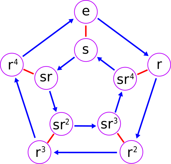
The dihedral group $D_5$: Do not get confused, the notation for “s” und “r” is exactly the other way around as in my text
Altogether there are $ |G|= 2N $ group elements, which are generated by $ N $ rotations $ s $ and a reflection about a fixed axis $ r $. Thus we can write any group element in the form
$$
s^x r^a \quad \text{with $ x \in \mathbb{Z}_N $ and $ a \in \mathbb{Z}_2 $}
$$
By our knowledge about 2d-rotations and reflections, we know, that the group operation is given by:
$$
s^x r^a \cdot s^y r^b = s^{x + (-1)^a y} r^{a+b}
$$
Aquivalently we may express this as the “semidirect product” $ (x, a), (y, b) \in \mathbb{Z}_N \rtimes \mathbb{Z}_2 $ and
\begin{gather}
(x, a) \cdot (y, b) = (x + (-1)^a y, a+b) \\
\text{and} \\
(x, a)^{-1} = (−(−1)^a x, a)
\end{gather}
where the weird $\rtimes$-sign expresses the fact the combination of elements is given by the latter relation and is not just a simple product.
5.7 Example: Fourier Sampling the Dihedral Group D4
Another very comprehensive investigation of the quantum computing framework for the hidden subgroup problem is the master thesis “The Hidden Subgroup Problem” by Frédéric Wang xii.
In there, Wang also presents an example of the different irreducible representations and measurement probabilities for weak and strong Fourier sampling outcomes for subgroups of $D_4$.
Representations
| $ \sigma $ | $ \sigma(x, 0)$ | $ \sigma(x, 1)$ |
|---|---|---|
| $ \sigma_0 $ | $ 1 $ | $ 1 $ |
| $ \sigma_1 $ | $ 1 $ | $ -1 $ |
| $ \sigma_2 $ | $ (-1)^x $ | $ (-1)^{x+1} $ |
| $ \sigma_4 $ | $$ \begin{pmatrix} (-1)^x & 0 \\ 0 & i^x \\ \end{pmatrix} $$ |
$$ \begin{pmatrix} 0 & (-i)^x \\ i^x & 0 \\ \end{pmatrix} $$ |
As for weak and strong Fourier sampling, Wang compares two different subgroups of $ D_4 $:
\begin{gather}
H_1 = \bigl\{(0, 0), (1, 1)\bigr\} \\
\text{and} \\
H_2 = \bigl\{(0, 0), (2, 0)\bigr\}
\end{gather}
Weak Fourier Sampling
For weak Fourier sampling this gives:
| $ \sigma $ | $ \sigma(H_1)$ | $ P(H_1, \sigma)$ | $ \sigma(H_2)$ | $ P(H_2, \sigma)$ |
|---|---|---|---|---|
| $ \sigma_0 $ | $ \sqrt{2} $ | $ \frac{1}{4} $ | $ \sqrt{2} $ | $ \frac{1}{4} $ |
| $ \sigma_1 $ | $ 0 $ | $ 0 $ | $ \sqrt{2} $ | $ \frac{1}{4} $ |
| $ \sigma_2 $ | $ 0 $ | $ 0 $ | $ \sqrt{2} $ | $ \frac{1}{4} $ |
| $ \sigma_3 $ | $ \sqrt{2} $ | $ \frac{1}{4} $ | $ \sqrt{2} $ | $ \frac{1}{4} $ |
| $ \sigma_4 $ | $$ \frac{1}{\sqrt{2}} \begin{pmatrix} 1 & -i \\ i & 1 \\ \end{pmatrix} $$ |
$ \frac{1}{2} $ | $$ \begin{pmatrix} 0 & 0 \\ 0 & 0 \\ \end{pmatrix} $$ |
$ 0 $ |
Strong Fourier Sampling
Since the first 4 representations are 1-dimensional, there will be no difference in weak and strong for those. Only sampling outcomes for $ \sigma_4 $ will give finer grained information for strong Fourier sampling this gives:
| $ (\sigma, j) $ | $ P(H_1, \sigma, j)$ | $ P(H_2, \sigma, j)$ |
|---|---|---|
| $ (\sigma_4, 1) $ | $ \frac{1}{4} $ | $ 0 $ |
| $ (\sigma_4, 2) $ | $ \frac{1}{4} $ | $ 0 $ |
5.8 Entangled measurements and the Kuperberg sieve
It can shown, that the dihedral hidden subgroup problem reduces to subgroups of type:
$$
H = \bigl\{(0, 0), (y, 1) \bigr\} \quad \text{for some $ y \in \mathbb{Z}_N$}
$$
Note, that $ (y, 1) $ is self inverse by the former relation.
Thus, the hidden subgroup problem for $ D_N $ reduces to find a hidden “slope” $ y $. For simplicity, let’s assume the case $ N = 2^n $. Setting up our quantum computing framework for the dihedral hidden subgroup problem will give us coset states of the form:
$$
U(z) \lvert H \rangle = \frac{1}{\sqrt{2}} \big( \lvert z, 0 \rangle + \lvert z + y, 1 \rangle \big)
$$
Solving this for $ y $ is also called the “Dihedral Coset Problem (DCP)”. Following an insight by Greg Kuperberg, this can be done in a little different way than in the standard approach xiii.
First we $\mathbb{Z}_N$-Fourier transform only the first register. This gives a superposition of states of the form
\begin{gather}
\lvert k \rangle \otimes \lvert \psi_k \rangle \\
\text{with} \\
\lvert \psi_k \rangle =
\frac{1}{\sqrt{2}} \big( \lvert 0 \rangle + e^{2\pi i \cdot \frac{k}{N} y} \lvert 1 \rangle \big)
\end{gather}
Now, we measure the $ \lvert k \rangle $-register. If we could generate / postselect states with $ k = N/2 $, we would end up with:
$$
\lvert \psi_{N/2} \rangle =
\frac{1}{\sqrt{2}} \big( \lvert 0 \rangle + (-1)^y \lvert 1 \rangle \big)
$$
If we measure such a state in the X-basis $ \lvert \pm \rangle = (\lvert 0 \rangle \pm \lvert 1 \rangle)/\sqrt{2}$ we would learn if $ y $ is even or uneven (its “parity”). This parity is nothing else than the last bit of $ y $ or its “least significant” bit. Kuperberg realized, that you could use this procedure to iteratively learn the last bit, the second last bit, the third last bit, … until you have learned all bits of the hidden slope $ y $. This is possible, because the dihedral group $ D_N $ is recursively self-similar: It contains two subgroups that are isomorphic to $ D_{N/2} $
\begin{gather}
\big\{(2x, 0), (2x, 1) : x \in Z_{N/2} \big\} \\
\big\{(2x, 0), (2x + 1, 1) : x \in Z_{N/2} \big\}
\end{gather}
If the parity of $ y $ is even, than the hidden subgroup is part of the former and if the parity of $ y $ is uneven, than the hidden subgroup is part of the latter. But this recursive group setup sais even more: If we simply drop a certain bit (respectively one certain qubit) from our coset state in the $\mathbb{Z}_N$-register, we get a new dihedral $(n-1)$-bit coset state which entirely lives in the even or in the uneven subgroup. And the bit, that we have to drop is the same parity-bit, that we just learned for our hidden slope $y$. The new coset state contains a new hidden subgroup with hidden slope $ y’ $. Just like the new coset state, the new slope is the string of the remaining $n-1$ bits and its new parity bit is the second last bit of $y$. Thus, by repeating this procedure we are able to learn all bits of the hidden slope $y$.
But …
… we still need to figure out, how to generate the state $ \lvert \psi_{N/2} \rangle $!
For one thing: Since we measure the $ \lvert k \rangle $-register, we may hope to draw a $ k = N/2 $. But since $ N = 2^n $ this is exponentially unlikely.
Kuperberg’s insight was, to entangle two such states $ \lvert \psi_p \rangle $ and $ \lvert \psi_q \rangle $ via a Controlled NOT. This gives a state of the same kind:
$$
\lvert \psi_p, \psi_q \rangle = \frac{1}{\sqrt{2}}
\big( \lvert \psi_{p+q} \rangle \lvert 0 \rangle + \alpha \cdot \lvert \psi_{p-q} \rangle \lvert 1 \rangle \big)
$$
with some irrelevant phase $ \alpha $. After measuring the second register, we get states of type $ \lvert \psi_{p+q} \rangle $ or $ \lvert \psi_{p-q} \rangle $. Remember that we know $ p $ and $ q $, since we measured this register after the Fourier transform before. Now, we can think of a whole bunch of clever ways to pair $ p $ and $ q $ according to their bitstrings, so that after the entangled measurement, we get a similar state with more zeros in their bitstrings. We can use such new states, that after yet another entangled measurement, we would get other similar states with even more zeros in their bitstrings. Thus by collecting states, measuring their Fourier labels, clever pairing and repeating entangled measurements we are able to generate a sequence of states that pretty soon end up with $ \lvert \psi_{N/2} \rangle $:
$$
\lvert \psi_{k} \rangle = \lvert \psi_{******} \rangle \longrightarrow \lvert \psi_{*****0} \rangle
\longrightarrow \lvert \psi_{****00} \rangle
\longrightarrow …
\longrightarrow \lvert \psi_{*00000} \rangle = \lvert \psi_{N/2} \rangle
$$
5.9 Lattice cryptography and the Dihedral Hidden Subgroup Problem
To complete this overview of the hidden subgroup problem, we will look into a highly interesting application of the dihedral hidden subgroup problem. It was discovered by Oded Regev in 2003 xiv. In particular, he reduced certain “shortest vector problems” (SVP), that occur in lattice cryptography, to the dihedral hidden subgroup problem.
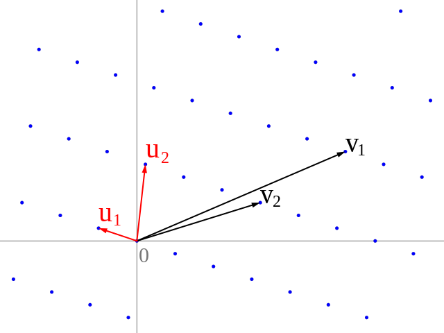
Image by Catslash via Wikimedia
A mathematical lattice is a periodic set of vectors in $ \mathbb{R}^n $, that is integer-spanned by a few basis vectors $ v_k $. These basis vectors might not be particularly short. A very well studied problem is the question for the shortest vector in the whole lattice (SVP). The larger the dimension of the lattice gets, the harder this shortest vector problem becomes. All known algorithms of the SVP have an exponential runtime, making it a great candidate for cryptography. In his seminal work Regev proved that finding this shortest vector may be reduced to the problem of finding the hidden slope in a dihedral hidden subgroup problem. The dihedral coset problem, that we examined in the previous section, can be extended to the “two point problem” of finding the minimal distance between two vectors $\vec{x}$ and $\vec{y}$ in a lattice via a collection of states of the form:
$$
\frac{1}{\sqrt{2}} \big( \lvert \vec{x}, 0 \rangle + \lvert \vec{y}, 1 \rangle \big)
$$
This sounds surprising at first, because here we are dealing with vectors. But the problem may be cast to an integer problem by chaining the integer components $ x_i – y_i $ of the distance vector to a b-adic representation (with a certain base $ M $), which is the hidden slope to be found:
$$
\sum_{i=1}^n(x_i – y_i) \cdot (2M)^{i-1}
$$
By knowing $M$ and this value, we are able to read off the integer components of the distance vector. Since we also know the basis of the lattice, we have solved the two point problem.
An essential part of Regev’s solution to the shortest vector problem is to partition the lattice into labeled elementary cubes, in such a way, that each cube contains either no lattice points or exactly two nearest lattice points. This can actually be done without knowing the shortest vector upfront. By storing the label of each cell in an ancillary register, the superposition of all lattice points will collapse to the points of exactly one elementary cube with two nearest points after measuring this register.
A nice introduction to this subject may be found here xv.
By the way: Just two years later Regev introduced the “Learning with Errors” Problem (LWE), which started a revolution in cryptography xvi.
In 2018, he was honored with the Gödel-Prize for his work.
6 Appendix 1: Some facts about group and representation theory
6.1 Groups
Of course, a “group” is a set $ G $ with an operation that maps every pair of elements into the set again $ g_1 \cdot g_2 \in G $. For every element $g$ there is also an “inverse” element $g^{-1} $ mapping $ g $ to the “neutral” element $ e $ which is also part of the group. The group is called “abelian” if the operation commutes for all elements. In this case the group operation is sometimes called $ + $, as we will also do.
The number of all elements in G (its “order”) is denoted as $ | G | $.
6.2 Examples
Example $ \mathbb{Z}_2^n $:
The set of bitstrings of length $ n $ forms the “cyclic group” $ \mathbb{Z}_2^n $ under the modulo addition: e.g. $ 01011 + 00001 = 01010 $ or $ 11111 + 00001 = 11110 $.
Example $ \mathbb{Z}_{2^n} $:
Of course, the same set of bistrings may also be interpreted in other ways, i.e. as the group $ \mathbb{Z}_{2^n} $: The set of integers $ 0, 1, …, 2^n-1 $ which repeat in a cyclic way again at $0$ just like the hours of a clock. The same bitstrings just map to a different element under addition / group operation: $ 01011 + 00001 = 01100 $ or e.g. $ 11111 + 00001 = 00000 $.
6.3 Subgroups
A subset $ H \subset G $ is a “subgroup”, if it also has all the group properties and all of $ H \cdot H $ stays in $ H $. Note, that the subgroup $ H = \bigl\{0, b \bigr\} $ from Simon’s problem is a subgroup of $ \mathbb{Z}_2^n $.
A “coset” is a set of type $ g \cdot H $ or $ g + H $ for a subgroup H and any $ g \in G $.
By “Lagrange’s theorem”, there are $ | G | / | H | $ distinct cosets.
Probably you knew all of this already. But the next section about representations might be less familiar …
BTW: A nice, short and rather gentle introduction can also be find here xvii.:
6.4 Representations
A “representation” $ \rho $ of a group is a way to encode the group elements as complex and invertable $N \times N$ matrices. Further it has to be a “group homomorphism”
\begin{gather}
\rho: G \longrightarrow GL \bigl(\mathbb{C}^N \bigr) \\
\rho(g_1 \cdot g_2) = \rho(g_1) \cdot \rho(g_2)
\end{gather}
So $\rho$ translates the group operation into ordinary matrix multiplication.
If $G$ is abelian this has some interesting consequences: Since
\begin{gather}
\rho(g_1 + g_2) = \rho(g_1) \cdot \rho(g_2) \\
= \rho(g_2 + g_1) = \rho(g_2) \cdot \rho(g_1)
\end{gather}
all the matrices in $ \rho(G) $ commute. That means, they have a common eigenbasis and there exists an invertable matrix $ V $ such that
\begin{gather}
V \cdot \rho(g) \cdot V^{-1} \quad \text{is diagonal for all $ g \in G $.}
\end{gather}
6.5 Irreducible Representations
In the abelian case above, the diagonal elements for each $ g \in G $ are different complex numbers $ \sigma(g) $.
Since $ V \cdot \rho \cdot V^{-1} $ is also a homomorphism and thus a representation, so are all the $ \sigma $. We see, that $ V \rho V^{-1} $ is “reducable”: It may be decomposed into smaller “irreducible representations” $ \sigma $ and so does $ \rho $.
A key insight of representation theory is, that any representation may be decomposed in this way into irreducible representations. For abelian groups these are just homomorphism functions
\begin{gather}
\sigma: G \longrightarrow \mathbb{C} \quad \text{abelian}
\end{gather}
and there are $ |G| $ different ones.
In general, for non-abelian groups, the $ \sigma $ map to small $d_\sigma \times d_\sigma$ matrices with individual dimension $ d_\sigma $.
\begin{gather}
\sigma: G \longrightarrow GL \bigl(\mathbb{C}^{d_\sigma} \bigr) \quad \text{non-abelian}
\end{gather}
Also in gernal, there are less such irreducible representations, usually denoted as $ \sigma \in \hat{G} $. But all degrees of freedom (labels and matrix indices) still add up to |G|:
\begin{gather}
\sum_{\sigma \in \hat{G}} d_\sigma^2 = |G|
\end{gather}
So, as the number of irreducible representations reduce, their sizes increase. In other words: The diagonal block structure of the group representations becomes coarser.
6.6 Characters
Now to the before mentioned “characters”: You may construct an interesting group function if you take the trace of a representation.
\begin{gather}
\chi(g) = Tr( \rho(g) )
\end{gather}
Thus, a character has the nice symmetrical property that it is constant on “conjugacy classes” for every subgroup $H$. This means, elementwise we have (because traces are cyclic):
\begin{gather}
\chi(g \cdot H \cdot g^{-1} ) = \chi(H)
\end{gather}
Also, you may extract some central properties of any group just by studying the characters and especially the characters of irreducible representations
\begin{gather}
\chi(g) = Tr( \sigma(g) )
\end{gather}
For abelian groups these characters are of course just the irreducible representations themselfs. So, they have the homomorphism property
\begin{gather}
\chi_z(g_1 + g_2) = \chi_z(g_1) \cdot \chi_z(g_2)
\end{gather}
7 Appendix 2: Fourier sampling the abelian coset state in detail
In this appendix we will carry out the calculation for the Fourier transform of an abelian coset state in detail. I will closely follow the presentation in Andrew Childs’ great “Lecture Notes on Quantum Algorithms” (chapter 6)
\begin{align}
\lvert \psi_5 \rangle &= \mathcal{F} \lvert g + H \rangle \\
&= \frac{1}{\sqrt{|H|\cdot|G|}} \cdot \sum_{k \in G} \sum_{h \in H} \chi_k(g + h) \lvert k \rangle \\
&= \sqrt{\frac{|H|}{|G|}} \cdot \sum_{k \in G} \chi_k(g) \cdot \chi_k(H) \lvert k \rangle
\end{align}
using the definition:
\begin{gather}
\chi_k(H)
:= \frac{1}{\sqrt{|H|}} \cdot \sum_{h \in H} \chi_k(h)
\end{gather}
Now, this latter sum is highly interesting:
I claim: If you sum up $\chi_k$ like this (over all elements of a group or a subgroup), then every $\chi_k$ will cancel out to $ 0 $ except for those, that are trivial $\chi_k = 1 $ on the group or subgroup!
Why so?
Let’s select a random $ h’$ and take a closer look at $ \chi_k(h’) $.
\begin{align}
\chi_k(H)
&= \frac{1}{\sqrt{|H|}} \cdot \sum_{h \in H} \chi_k(h) \\
&= \frac{1}{\sqrt{|H|}} \cdot \sum_{h \in H} \chi_k(h + h’) \\
&= \frac{1}{\sqrt{|H|}} \cdot \chi_k(h’) \cdot \sum_{h \in H} \chi_k(h) \\
&= \chi_k(h’) \cdot \chi_k(H)
\end{align}
This is only possible if $ \chi_k(h’) = 1 $ or $ \chi_k(H) = 0$.
This leaves us with:
\begin{gather}
\lvert \psi_5 \rangle
= \sqrt{\frac{|H|}{|G|}} \cdot \sum_{k: \chi_k(H) = 1} \chi_k(g) \lvert k \rangle
\end{gather}
8 Appendix 3: Strong and Weak Fourier sampling in detail
In the main text we saw, that Fourier transforming a non-abelian coset state gives us:
\begin{align}
\mathcal{F}_{\sigma} \lvert g’ \cdot H \rangle
&= \sqrt{\frac{d_{\sigma}}{|G|}} \cdot \sum_{i, j \leq d_{\sigma}} \sigma(g’ \cdot H)_{i, j} \cdot \lvert \sigma, i, j \rangle \\
&= \sqrt{\frac{d_{\sigma}}{|G|}} \cdot \sum_{i, j \leq d_{\sigma}} \big( \sigma(g’) \cdot \sigma(H)\bigr)_{i, j} \cdot \lvert \sigma, i, j \rangle
\end{align}
where we have used the definition $ \sigma(g’ \cdot H) := \frac{1}{\sqrt{|H|}} \sum_{h \in H} \sigma(g’ \cdot h) $
8.1 Strong Fourier sampling in detail
The probability to measure $\sigma, i, j$ for the coset state $\lvert g’ \cdot H \rangle $ still depends on $ g’ $:
$$
P(g’, \sigma, i, j ) = \frac{d_{\sigma}}{|G|} \cdot \big| \big( \sigma(g’) \cdot \sigma(H)\bigr)_{i, j} \big|^2
$$
This looks disappointing. But we are still able to get rid off $ g’$! Since the second register, the one for our blackbox function, will collapse into arbitrary $ g’$-images in each iteration, we practically sample uniformly from all $ g’ \in G $! Thus, if we just keep measuring $ \sigma, i, j $, this will give us the mean average $ \frac{1}{|G|} \sum_{g’ \in G} $:
$$
P(\sigma, i, j ) = \frac{d_{\sigma}}{|G|} \cdot \frac{1}{|G|} \sum_{g’ \in G} \big| \big( \sigma(g’) \cdot \sigma(H)\bigr)_{i, j} \big|^2
$$
If we write the matrix multiplication in detail, we get:
$$
P(\sigma, i, j ) = \frac{d_{\sigma}}{|G|^2} \cdot \sum_{g’ \in G} \big| \sum_{k=1}^{d_\sigma} \big( \sigma(g’) \big)_{i,k} \cdot \big( \sigma(H)\bigr)_{k, j} \big|^2
$$
Oh no, this looks even messier!
But don’t get confused with all the notations. The key to success here, is the observation that for each $k$, $ \big( \sigma(g’)_{i,k} \big)_{g’} =: \big(v_k \big)_{g’} $ may be interpretated as a $ |G| $-dimensional vector $ v_k $ with index $ g’$. To simplify the sum, we ignore $ i, j $ for a second and also define the complex coefficients $ \gamma_k := \sigma(H)_{k, j} $.
This makes the sum:
$$
P(\sigma, i, j ) = \frac{d_{\sigma}}{|G|^2} \cdot \sum_{g’ \in G} \big| \sum_{k=1}^{d_\sigma} \big(v_k \big)_{g’} \cdot \gamma_k \big|^2
$$
Now, think about the following claim for a second: This is nothing else than the norm of the superposition of the vectors $ (v_k) $ in the |G| dimensional vector space with index $g’$! So we get rid off the first sum:
$$
P(\sigma, i, j ) = \frac{d_{\sigma}}{|G|^2} \cdot
\left\lVert \sum_{k=1}^{d_\sigma} \big(v_k \big) \cdot \gamma_k \right\rVert^2
$$
Note, that these vectors are not quantum states (we just measured one). The norm of the $ |G| $-dimensional vector is just a way of interpreting the distribution. Since it is not a quantum state, we will omit the bracket notation. This norm simplifys further, by the observation, that the vectors $ \big(v_k \big) $ are orthogonal for all $ k $ by Schur’s lemma (the orthogonal relation for the $\sigma$’s).
Now, if you make a superposition of any set of orthogonal vectors by some coefficients, what is the norm of this? The norm is just the squares of the coefficients $ \gamma_k $ times the inner product of the vectors $ \langle v_k, v_k \rangle $ (in this case, given by Schur’s lemma again)! No matter how large the vectors are and what the vector space is. All that counts, is that they are orthogonal. So the sum simplifies to:
\begin{align}
P(\sigma, i, j ) &= \frac{d_{\sigma}}{|G|^2} \cdot
\sum_{k=1}^{d_\sigma} | \gamma_k |^2 \cdot \frac{|G|}{d_{\sigma}} \\
&= \frac{1}{|G|} \cdot
\sum_{k=1}^{d_\sigma} | \sigma(H)_{k, j} |^2 \\
&= \frac{1}{|G|} \cdot \lVert \sigma(H)_j \rVert^2
\end{align}
where $ \lVert \sigma(H)_j \rVert $ is the norm of the j’th column vector of $ \sigma(H) $.
This shows in detail, that the probability $ P(\sigma, i, j ) $ is constant on the row register $ i $ and independent on any translation by $ g’ $.
8.2 Weak Fourier sampling in detail
If we only care about measuring the Fourier labels, we need to sum over this distribution. Since the distribution is constant on $i$, the sum $ \sum_i $ will give us a constant factor $ d_\sigma $:
$$
P(\sigma) = \sum_{i,j=1}^{d_\sigma} P(\sigma, i, j )
= \frac{d_\sigma}{|G|} \cdot \sum_{k, j=1}^{d_\sigma} | \sigma(H)_{k, j} |^2
$$
This sum is also a canonical norm for matrices, called the “Frobenius norm”, for which a nice trace equality holds:
$$
P(\sigma) = \frac{d_\sigma}{|G|} \|\sigma(H) \|_F^2 =
\frac{d_\sigma}{|G|} Tr \big( \sigma(H)^\dagger \cdot \sigma(H) \big)
$$
This may be simplified further. Recalling our trick for abelian Fourier sampling,
$$
\sigma(H) = \sigma(h) \cdot \sigma(h^{-1}H) = \sigma(h) \cdot \sigma(H)
$$
we might be tempted to conclude, that $ \sigma(h) = 1 ? $ and we will Fourier sample only those $ \sigma $’s that are trivial on $ H $. But what is true for complex numbers does not necessarily hold for matrices as well. All that the equation above tells us is:
$$
\sigma(H) \cdot \sigma(H) = \frac{1}{\sqrt{|H|}} \sum_{h \in H} \sigma(h) \cdot \sigma(H) = \frac{|H|}{\sqrt{|H|}} \cdot \sigma(H) = \sqrt{|H|} \cdot \sigma(H)
$$
Thus $ \sigma(H) $ is proportional to a projection matrix (and each $ \sigma(h) $ might be non trivial on the kernel of $ \sigma(H) $). We may use the equation above to simplify the Frobenius norm. Since $ \sigma(H)^\dagger = \sigma(H^{-1}) = \sigma(H) $ (think of this as written in sums):
\begin{align}
P(\sigma) &= \frac{d_\sigma}{|G|} \cdot Tr \big( \sigma(H)^\dagger \cdot \sigma(H) \big) \\
&= \sqrt{|H|} \cdot \frac{d_\sigma}{|G|} \cdot Tr \big( \sigma(H) \big)
\end{align}
9 Footnotes
i https://arxiv.org/abs/2209.06930: “How Much Structure Is Needed for Huge Quantum Speedups?” Transcript of Scott Aaronson‘s talk at the Solvay Physics Conference in Brussels, May 2022.
ii https://arxiv.org/abs/2212.08678: “A super-polynomial quantum advantage for combinatorial optimization problems” paper by N. Pirnay, V. Ulitzsch, F. Wilde, J. Eisert, J. Seifert 2022
iii https://arxiv.org/abs/2010.02174: “A rigorous and robust quantum speed-up in supervised machine learning” 2010, paper by Y. Liu, S. Arunachalam, K. Temme. It creates a very nice machine learning example with data that a classical computer can easily generate by modular exponentiation but cannot classify / distinguish from random data due to the classical hardness of discrete logarithms whereas the quantum support vector machine can.
iv https://arxiv.org/abs/2210.07234: “The Complexity of NISQ” 2022, paper by S. Chen, J. Cotler, HY. aka Robert Huang, J. Li one of the highest SciRated preprints in quantum computing in the last year. It introduces a new complexity class for NISQ-algorithms and proves that there exists an exponential oracle seperation between BPP, NISQ and BQP (in this order).
v https://qiskit.org/textbook/ch-algorithms/simon.html: You will find a very similar introduction to Simon’s problem and a nice coding example in the Qiskit Textbook
vi https://arxiv.org/abs/quant-ph/9803072: Ekert & Jozsa 1998, “Quantum Algorithms: Entanglement Enhanced Information Processing”, which also gives details about the general Fourier transform over finite groups
vii https://www.quantamagazine.org/finally-a-problem-that-only-quantum-computers-will-ever-be-able-to-solve-20180621/: “Finally, a Problem That Only Quantum Computers Will Ever Be Able to Solve”, a nice article on Quantamagazine about the Forrelation problem and the breakthrough in quantum complexity theory. There, you will also find a link to the preprint.
viii http://www.cs.umd.edu/~amchilds/qa/: Andrew Childs’ truly great “Lecture Notes on Quantum Algorithms” and a very comprehensive reference for the hidden subgroup problem
ix https://arxiv.org/abs/quant-ph/0012084: Richard Jozsa 2000, “Quantum factoring, discrete logarithms and the hidden subgroup problem”
x https://dl.acm.org/doi/10.1145/380752.380769: M. Grigni et al. 2001, “Quantum mechanical algorithms for the nonabelian hidden subgroup problem”
xi https://arxiv.org/abs/quant-ph/0511148, S. Hallgren et al 2005. “Limitations of Quantum Coset States for Graph Isomorphism”
xii https://arxiv.org/abs/1008.0010, F. Wang’s master thesis. 2010 “The Hidden Subgroup Problem”, a very comprehensive investigation about prior work on the subject.
xiii http://arxiv.org/abs/quant-ph/0302112, Greg Kuperberg 2003, “A subexponential-time quantum algorithm for the dihedral hidden subgroup problem.”. You will also find an introducation in Andrew Child’s lecture notes and F. Wang’s master thesis
xiv https://arxiv.org/abs/cs/0304005, Oded Regev 2003, “Quantum Computation and Lattice Problems”
xv https://cbright.myweb.cs.uwindsor.ca/reports/cs667proj.pdf, Curtis Bright, 2009 “From the Shortest Vector Problem to the Dihedral hidden subgroup problem”
xvi https://dl.acm.org/doi/10.1145/1060590.1060603, Oded Regev 2005 “On lattices, learning with errors, random linear codes, and cryptography”
xvii
http://buzzard.ups.edu/courses/2010spring/projects/roy-representation-theory-ups-434-2010.pdf, Ricky Roy, “Representation Theory”, A nice, short and rather gentle introduction